This is the plain-language version of the paper "When does training on downscaled images yield the same gradients?" (arXiv:2608.04448). The paper has 80 KB of appendix; this post has none. If a number below feels under-justified, the appendix is where the justification lives.

The idea, and why it isn't obviously fine

A diffusion transformer pays for resolution twice. Token count grows with the square of the edge length, and attention grows with the square of the token count. A 1024-tier image is ~4,100 latent tokens; 896 is ~3,000; 768 is ~2,160; 512 is ~1,000. Every step you can run on a smaller grid is a step that is noticeably cheaper.

And there's a well-known reason to think some steps can be run smaller. Flow-matching training noises the latent as $z_\sigma = (1-\sigma)x + \sigma\epsilon$. At high $\sigma$ the fine spatial frequencies are the first to drown in the noise, so above some crossover a downscaled latent carries almost all of the signal that survives anyway. The inference-side literature (scale-wise distillation, spectral progressive diffusion, spectrally-guided schedules) already runs high-noise sampling steps at low resolution on exactly this premise.

So the proposal, which I call demotion, is: keep the model, the loss, and the $\sigma$ distribution unchanged; on some steps, replace the native latent with one encoded from a downscaled version of the same image; train the LoRA as usual.

1  σ ~ p_train
2  x ← native latent of y
3  if σ > σ* and y on-route:          # the whole change is lines 3–5
4      x ← demoted latent of y
5      rotary ← banded(σ)             # optional refinement
6  ε ~ N(0, I) at shape(x)
7  z ← (1−σ)x + σε
8  v ← ε − x
9  step on ‖v̂(z, σ, c) − v‖²

The question is whether the gradient you get on line 9 points the same way it would have pointed on the native grid. The spectral argument says yes, once the noise has masked the frequencies the coarse grid throws away. But that argument is a statement about the data, and a training step is not just data. Written out, the per-step adapter gradient is

$g = J^{\top} r,$

the network Jacobian times the prediction residual. Demotion touches both factors: the residual, because the target $v = \epsilon - x$ carries the clean image at full weight at every noise level (noise never masks the target), and the Jacobian, because the compute graph itself changes when you change the grid: fewer tokens in every softmax, and rotary position embeddings that accumulate phase at a different density across the image. The spectral picture has nothing to say about the second factor at all.

So instead of trusting the premise, I measured the thing directly.

The instrument: comparing gradients, not samples

The estimand is simple. For a (image, caption) pair and a noise bin $\sigma$, average the LoRA gradient over many noise draws on the native latent, do the same on the demoted latent, and take one minus the cosine between the two:

$d_e(\sigma) = 1 - \cos\big(\bar g_{\text{src}}(\sigma),\ \bar g_{\text{dem}}(\sigma)\big).$

Zero means "same direction". A control arm, reenc, decodes and re-encodes the native latent through the VAE without changing the grid, so its distance prices the VAE round trip alone; everything reported below is the excess over that control, i.e. the part of the gap you can attribute to the grid change. The verdict run used 40 images, 12 noise draws per bin, 14 bins across $(0,1)$ plus a $\sigma=1$ endpoint, on Anima (2B DiT, 28 blocks, 3D RoPE, Qwen-Image VAE) with a plain LoRA trained at native tiers.

One thing bit me hard here and is worth a paragraph. A finite-draw average is the true mean plus noise, and noise is (on average) orthogonal to the mean, so every finite-draw cosine is attenuated below its population value. Worse, the attenuation is arm-dependent: per-draw gradient variance goes up as the token count goes down, so the coarser grid is attenuated more. The artifact this produces is a positive, $\sigma$-independent gap that grows as the target grid shrinks, which is exactly the signature of the effect I was trying to detect. The uncorrected $1024{\to}896$ endpoint gap read $+0.100/+0.035/-0.016$ at $D=4/8/16$ draws, a clean $c/D$ decay toward nothing. The fix is Spearman's 1904 correction for attenuation: run a second independent draw set for every arm, measure each arm's cosine with its own redraw, and divide:

$\hat c = \frac{\cos(g_{\text{src}}, g_a)}{\sqrt{\cos_{\text{self},\text{src}}\cdot\cos_{\text{self},a}}}.$

After debiasing, the fits come out flat in $D$, and extrapolating the native redraw floor gives a self-cosine of $1.005$ (CI $[0.994, 1.016]$): the population per-bin native gradient is a fixed direction, and the entire raw floor was draw noise. Half the "unsafe at every $\sigma$" verdict on the 768 route turned out to be this artifact. (Same lesson as the GPU-noise post: measure your null before you interpret your effect.)

The map

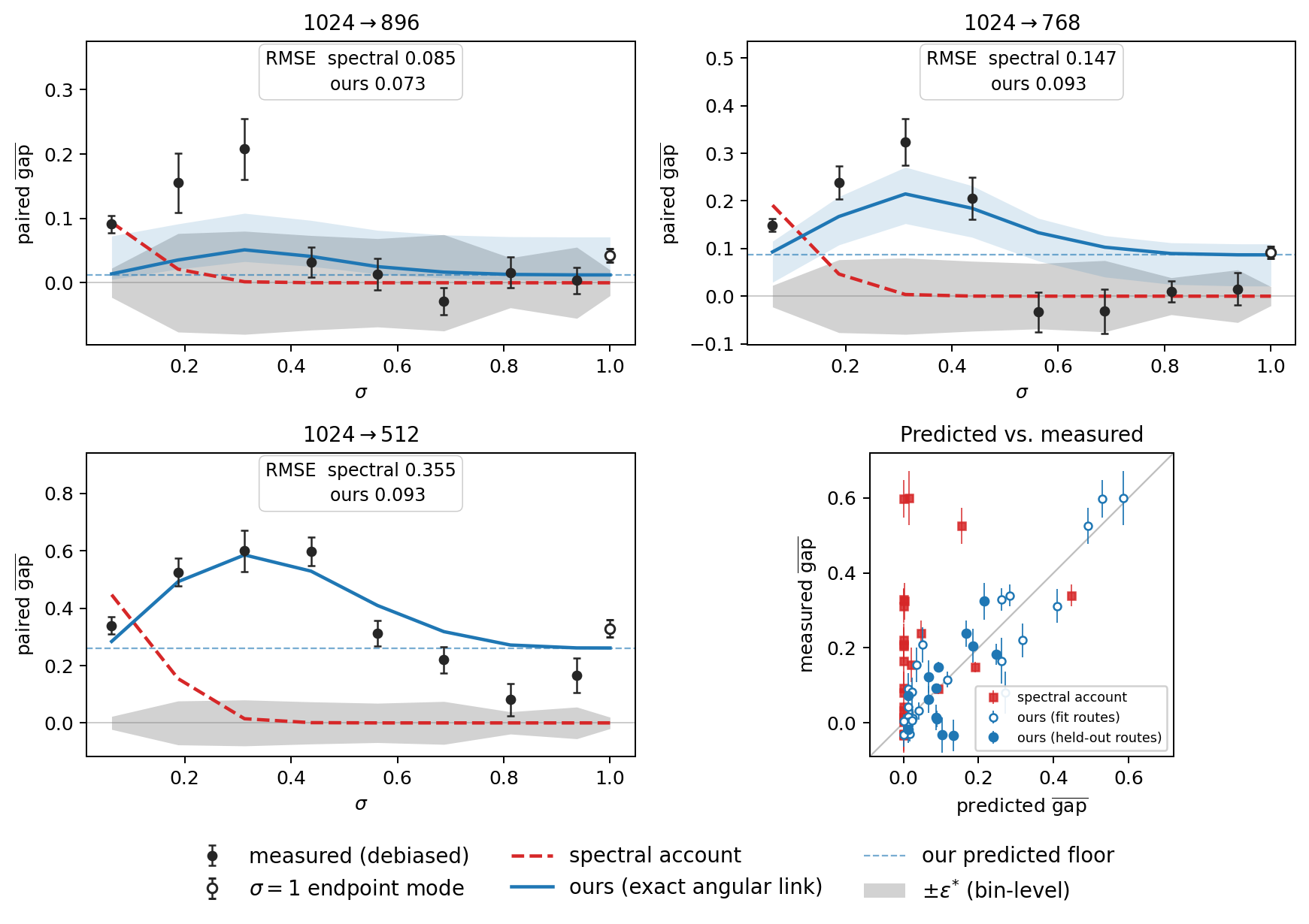
Black curves are the measured debiased excess per route; the gray band is the instrument's resolution per bin. Read against a pre-specified margin:

• $1024{\to}896$ is safe on $\sigma \in (0.5, 0.94]$, simultaneously over seven bins, with a floor of $0.02$–$0.04$. The $\sigma = 1$ endpoint carries a small real gap ($+0.02$–$0.03$) that raw estimation had buried under variance.
• $1024{\to}768$ is safe on no window at the strict margin, but has a narrow low-excess window $\sigma \in (0.65, 0.95)$ with excess $+0.02$–$0.04$, below the route's own floor. Hold that thought.
• Anything to 512 is unsafe in all fifteen bins, floor $\approx 0.30$.

Two things on this plot should bother anyone who believed the spectral story. First, the red dashed curves (the spectral prediction, transported into gradient units at its most favorable tolerance) sit near zero exactly where the measured curves peak, and predict zero above $\sigma \approx 0.15$–$0.20$ where a floor plainly persists. Second, the measured curves are not monotone: there is a mid-$\sigma$ cliff on 896 and a dip inside the 768 window that no "noise masks frequencies" argument can produce.

What actually governs the gap: ratio and token count

The blue curves are the account I ended up with. On the measured residual it reduces to two terms:

$\text{gap}_e(\sigma) \approx \underbrace{\tfrac12 a_e^2\,\big(\|\Delta\bar r(\sigma)\| / \|\bar g_{\text{src}}(\sigma)\|\big)^2}_{\text{data term}} + \underbrace{\text{RoPE}_e + \text{Resid}_e}_{\text{graph floor}}.$

The data term is a per-route amplitude on a universal mismatch curve: the mean prediction residual's cross-grid mismatch has the same monotone $\sigma$-shape on every route to within $\pm 0.02$, even across routes whose floors span $0$ to $0.3$. That is already a refutation of the diagonal spectral model, which says the mismatch should live in the destroyed band and be ordered by its energy. It isn't; all route identity lives in the Jacobian.

The floor is a $\sigma$-independent constant per route, and two probes say what sets what:

• Ratio sets the amplitude. A synthetic route $1280{\to}1120$, same edge ratio as $1024{\to}896$ at $1.6\times$ the absolute size, reproduces the $1024{\to}896$ curve bin for bin, crossover included.
• Absolute target size sets the floor. $896{\to}768$ has nearly the same ratio as $1024{\to}896$ but lands on a high-$\sigma$ residual ${\sim}2\times$ larger; meanwhile $1024{\to}768$ and $896{\to}768$, different ratios, same ${\sim}2{,}160$-token target, land on the same floor. The floor grows monotonically as the target grid shrinks: $0.02$–$0.04$ at ~3,000 tokens, $0.06$–$0.09$ at ~2,160, $\approx 0.30$ at ~1,000.

So the spectral argument isn't wrong about its own term: ratio really is the right governor for the data term. Its error is scope. It models one part of one branch of what demotion perturbs, and the part it leaves out is the one that never goes away no matter how much noise you add.

Where does the floor come from? Evaluate the demoted grid at positionally-interpolated fractional rotary coordinates, so its relative phase geometry matches native. That erases the 768 endpoint floor entirely and removes ~30% of the 512 floor. So on the 768 route the floor is essentially all RoPE; on 512 there's a genuine non-positional residue of ~0.2 left over, which I read as the coarse graph simply not having enough tokens to approximate the fine graph's computation.

The part I didn't expect: the gap is a residual of a near-cancellation

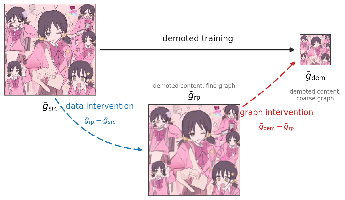
Demotion changes data and graph at once, and the trainer never realizes them separately. But there is an intermediate state you can train on: take the downscaled content and carry it back up to the native grid. Super-resolution people have trained on this (coarse content on the fine grid) since SRCNN. Call it the repromote arm. It changes the data without changing the graph, so it splits the perturbation into two legs:

$\delta g = \underbrace{(\bar g_{\text{rp}} - \bar g_{\text{src}})}_{B:\ \text{data}} + \underbrace{(\bar g_{\text{dem}} - \bar g_{\text{rp}})}_{C:\ \text{graph}}.$

This is an identity, not an approximation; all three live in the same adapter-parameter space. Measured as vectors, here is what the two legs look like:

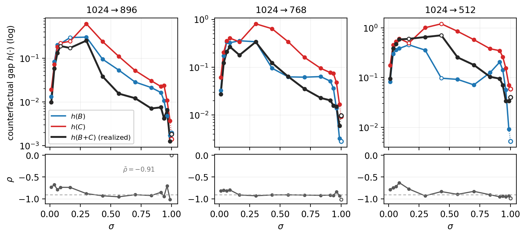
At every (route, $\sigma$) both branches alone are far larger than the realized gap. On the 896 route, the data branch by itself would produce $104$–$112\%$ of the measured plateau. The realized curve sits far below both because the two legs are deeply anti-aligned: $\rho = \cos(B^\perp, C^\perp)$ ranges $-0.63$ to $-0.96$ and pools to $\bar\rho = -0.91$. The cancellation removes $70$–$77\%$ of the summed branch cost on the safe routes.

In words: what demotion does to the data the objective consumes is nearly undone by what the changed compute graph does in response. The measured gap is not "how much the coarse grid hurts"; it is the leftover of a collision.

This explains the shapes the spectral account couldn't. Wherever the two legs' amplitude ratio passes through $1$ while the angle stays deep, the residual collapses below either branch alone, below even the route's floor. On 896, $|B^\perp|/|C^\perp|$ crosses $1$ within one bin of the mid-$\sigma$ cliff. On 768 it never quite crosses (rides at $0.76$–$0.88$ through the window), closest to balance exactly where the dip is. And 512 keeps the same deep angle ($|\rho| \approx 0.86$) but its amplitudes never balance: what fails on an unsafe route is magnitude matching, not the cancellation itself.

A few things about this geometry that I found genuinely surprising:

• It's born in the backward pass. The same decomposition at the residual level reads only $\rho_r = -0.12$ to $-0.22$. The deep anti-alignment appears when you pull back through $J^\top$; it is a property of the compute graph, not of the data statistics.
• It's everywhere. Resolved over 28 blocks and 15 module types, every gated cell reads $\rho$ in $-0.8$ to $-0.97$, cross-attention and MLPs included, with interquartile range $\le 0.11$. It isn't carried by a few modes; it holds pointwise in parameter space.
• RoPE phase misalignment is part of what makes the branches cancel. Fix the demoted graph's rotary phases to match native, and the graph branch rotates, the anti-alignment halves ($\rho \to -0.34$ to $-0.60$), and $h(C)$ doubles. With phases aligned, the graph branch stops magnitude-matching the data branch. So the "obvious" fix, uniform position interpolation, is off-manifold in-window. Only a frequency-selective (YaRN-style, $\sigma$-gated) alignment survived both pre-registered legs.
• The residual direction is a smooth $\sigma$-indexed axis field. At fixed $\sigma$, the 896 and 768 routes push the adapter along the same line (median $|\cos| = 0.95$–$0.97$), and the direction rotates smoothly with $\sigma$ with no sign flips. It's structure, not condition noise.
• It replicated on two further LoRAs of the same base model, trained on disjoint data along a designed style axis, at every bin of the 768 window. 896 replication is still an open cell.

Does it actually save anything?

Restricting demotion to the measured-safe route ($1024{\to}896$) above a one-sided gate ($\sigma > 0.5$), with no change to the objective, optimizer, or noise density, saves 14.6% training time at a fixed step budget on my corpora (15.1% of forward compute).

The more interesting question is what it does to the weights. I trained arms with deterministic kernels and paired RNG, so an identical retrain reproduces its twin at cosine $1.000$ and the only remaining reference noise is what non-deterministic kernels alone would introduce (the twin-pair floor from the other post):

Reading down: demoting at every $\sigma$ falls below the kernel-noise floor, i.e. it visibly moves the endpoint. Demoting only above the gate matches or exceeds that floor. Late scheduling brings the endpoint to cosine $0.75$–$0.77$ against native, at proportionally reduced saving. And stacking the 768 low-excess window onto the late rule, which the map predicted to be nearly free, is nearly free: the cosine doesn't move.

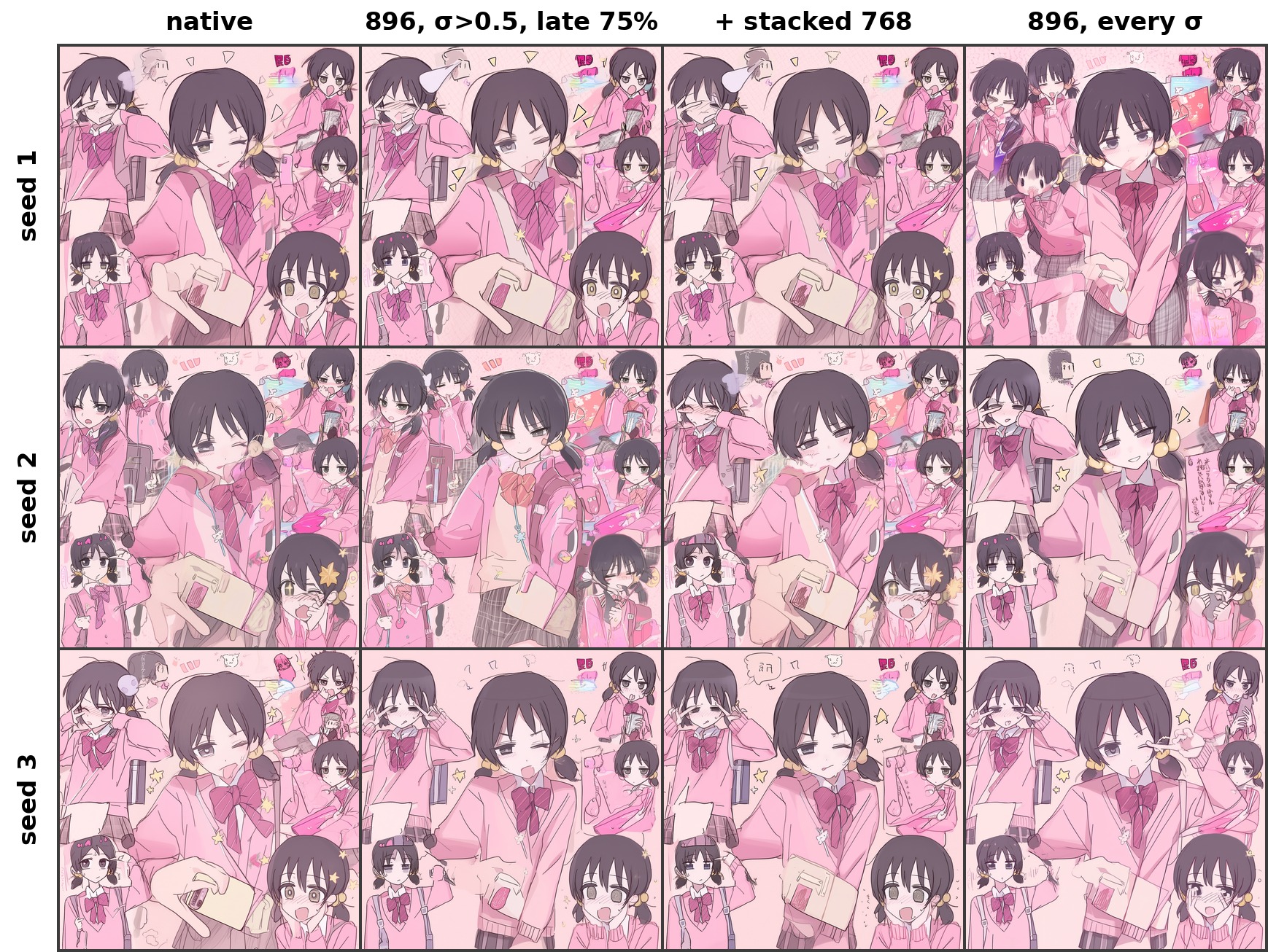
Columns are arms, rows are training seeds. Moving across a row (arm, fixed seed) changes the render about as much as moving down a column (seed, fixed arm); the gate-removed arm on the right drifts the most, matching its lowest cosine.

If you want to try this on your own model

The recipe is small, but the recipe is not the point. The point is that "train part of the time at lower resolution" proposals should pass a gradient-level test before you believe them, and the test is cheap: one probe run, a handful of arms, cosine of accumulated LoRA gradients per $\sigma$ bin, with the finite-draw correction. Concretely:

1. Don't use the spectral crossover as your gate. On this model it sits at $\sigma \approx 0.15$–$0.20$; the measured safe gate is $0.5$, and there's a floor above it that no $\sigma$ removes.
2. Watch the target's absolute token count, not the ratio. The floor is set by how many tokens you land on. ~3,000 was fine here; ~2,160 had a narrow window; ~1,000 was never safe.
3. Measure your null. Run a second independent draw set per arm and debias, or you will "discover" a floor that is just draw variance, or miss a real one.
4. Late-schedule it if you care about the endpoint. Demotion early in the run moves the weights more than demotion late.
5. Don't uniformly interpolate RoPE on demoted steps. The phase mismatch is doing some of the cancelling. Banded, $\sigma$-gated alignment is the version that held up.

What this doesn't cover

One model family (Anima), one adapter checkpoint trained at native tiers; a mixed-resolution-trained adapter might behave differently. The account predicts held-out routes at ${\sim}0.07$–$0.09$ RMSE, not within instrument resolution, and its ratio governor rests on two ratio values. The upper tail $\sigma \in (0.94, 1)$ is underpowered. The weight-space read is at 480 steps, not production scale. And the geometry names a family of levers (a per-$\sigma$-bin residual-direction guard, an explicit resolution conditioning of the phase-response pathway) that I have not tested; nothing above depends on them.

The full paper, with the appendix behind every number above, is on arXiv: arXiv:2608.04448.